Understanding Modern GPU Architecture and Parallel Computing

Introduction

Modern graphics processing units (GPUs) represent one of the most fascinating achievements in computer architecture. These devices can perform upwards of 36 trillion calculations per second - a scale so massive that it would require the population of 4,400 Earths working continuously to match this computational power. This article provides a deep technical analysis of GPU architecture, parallel computing paradigms, and practical implementations for leveraging this incredible processing power.

GPU vs CPU Architecture

Architectural Differences

The fundamental distinction between GPUs and CPUs lies in their architectural approach to computation:

1. Core Count and Specialization
   • GPUs: 10,000+ specialized cores optimized for parallel processing
   • CPUs: 8-24 complex cores optimized for sequential processing and task switching
2. Processing Paradigm
   • GPUs: Single Instruction, Multiple Data (SIMD) / Single Instruction, Multiple Threads (SIMT)
   • CPUs: Complex instruction set with branch prediction and out-of-order execution
3. Memory Architecture

   • GPUs: High-bandwidth memory with massive throughput (1.15 TB/s)

   • CPUs: Lower bandwidth but more flexible memory hierarchy (64 GB/s)

The Cargo Ship Analogy

Think of a GPU as a massive cargo ship and a CPU as a jumbo jet:

• GPU (Cargo Ship):
  • Huge cargo capacity (parallel processing)
  • Limited flexibility in routes (specialized instructions)
  • Slower but more efficient for bulk operations
• CPU (Jumbo Jet):
  • Smaller cargo capacity (sequential processing)
  • Highly flexible routing (general-purpose computing)
  • Faster for individual operations

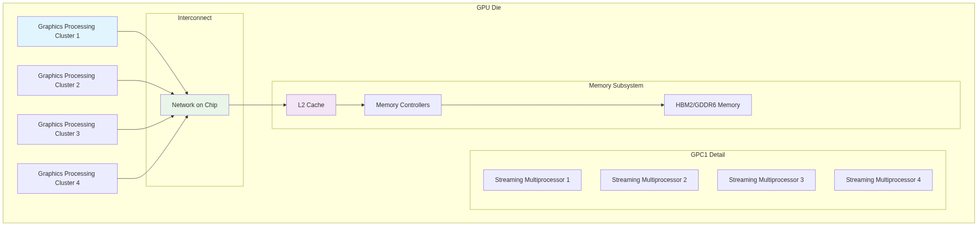
Physical Architecture of Modern GPUs

Hierarchical Organization

Modern GPUs follow a hierarchical organization:

1. Graphics Processing Clusters (GPCs)
   • Top-level organizational unit
   • Contains multiple Streaming Multiprocessors (SMs)
2. Streaming Multiprocessors (SMs)
   • Contains multiple warps and specialized cores
   • Includes shared memory and L1 cache
3. Warps
   • Group of 32 threads executed simultaneously
   • Basic unit of thread execution
4. Core Types
   • CUDA Cores: Basic arithmetic operations
   • Tensor Cores: Matrix operations
   • RT Cores: Ray tracing calculations

Implementation Example

Let’s implement a simple program that demonstrates the concept of parallel processing using OpenMP as an analogy for GPU processing:

#include <stdio.h>
#include <stdlib.h>
#include <omp.h>
#include <time.h>

#define ARRAY_SIZE 1000000
#define NUM_THREADS 8

void parallel_array_operation(float* input, float* output, int size) {
    #pragma omp parallel num_threads(NUM_THREADS)
    {
        int thread_id = omp_get_thread_num();
        int chunk_size = size / NUM_THREADS;
        int start = thread_id * chunk_size;
        int end = (thread_id == NUM_THREADS - 1) ? size : start + chunk_size;

        // Simulate GPU-like parallel processing
        for (int i = start; i < end; i++) {
            // Simple arithmetic operation
            output[i] = input[i] * 2.0f + 1.0f;
        }
    }
}

int main() {
    float *input = (float*)malloc(ARRAY_SIZE * sizeof(float));
    float *output = (float*)malloc(ARRAY_SIZE * sizeof(float));
    
    // Initialize input array
    srand(time(NULL));
    for (int i = 0; i < ARRAY_SIZE; i++) {
        input[i] = (float)rand() / RAND_MAX;
    }

    // Measure execution time
    double start_time = omp_get_wtime();
    parallel_array_operation(input, output, ARRAY_SIZE);
    double end_time = omp_get_wtime();

    printf("Execution time: %f seconds\n", end_time - start_time);
    printf("First 5 results: %f %f %f %f %f\n", 
           output[0], output[1], output[2], output[3], output[4]);

    free(input);
    free(output);
    return 0;
}

To compile and run this code:

gcc -fopenmp parallel_processing.c -o parallel_processing
./parallel_processing

The assembly output for the critical section (using gcc -S):

.L3:
    movss   (%rdi,%rax,4), %xmm0    # Load input value
    mulss   .LC0(%rip), %xmm0       # Multiply by 2.0
    addss   .LC1(%rip), %xmm0       # Add 1.0
    movss   %xmm0, (%rsi,%rax,4)    # Store result
    addq    $1, %rax                # Increment counter
    cmpq    %rdx, %rax              # Compare with end
    jl      .L3                     # Loop if not done

Computational Architecture and SIMD/SIMT

SIMD vs SIMT Architecture

SIMD (Single Instruction, Multiple Data)

• Traditional parallel processing model
• All threads execute exactly the same instruction
• Lock-step execution
• Limited flexibility with branching

SIMT (Single Instruction, Multiple Threads)

• Modern GPU architecture
• Threads can diverge and reconverge
• Individual program counters
• Better handling of conditional code

Let’s implement a SIMT-like operation in C:

#include <stdio.h>
#include <stdlib.h>
#include <pthread.h>
#include <time.h>

#define WARP_SIZE 32
#define NUM_WARPS 4
#define TOTAL_THREADS (WARP_SIZE * NUM_WARPS)

typedef struct {
    int thread_id;
    float* input;
    float* output;
    int size;
} ThreadData;

void* simt_thread(void* arg) {
    ThreadData* data = (ThreadData*)arg;
    int tid = data->thread_id;
    int stride = TOTAL_THREADS;
    
    // Simulate SIMT execution with divergent paths
    for (int i = tid; i < data->size; i += stride) {
        if (data->input[i] > 0.5f) {
            // Branch 1: Square the value
            data->output[i] = data->input[i] * data->input[i];
        } else {
            // Branch 2: Double the value
            data->output[i] = data->input[i] * 2.0f;
        }
    }
    
    return NULL;
}

int main() {
    const int size = 1024;
    float* input = (float*)malloc(size * sizeof(float));
    float* output = (float*)malloc(size * sizeof(float));
    pthread_t threads[TOTAL_THREADS];
    ThreadData thread_data[TOTAL_THREADS];
    
    // Initialize input array
    srand(time(NULL));
    for (int i = 0; i < size; i++) {
        input[i] = (float)rand() / RAND_MAX;
    }
    
    // Create threads
    for (int i = 0; i < TOTAL_THREADS; i++) {
        thread_data[i].thread_id = i;
        thread_data[i].input = input;
        thread_data[i].output = output;
        thread_data[i].size = size;
        pthread_create(&threads[i], NULL, simt_thread, &thread_data[i]);
    }
    
    // Join threads
    for (int i = 0; i < TOTAL_THREADS; i++) {
        pthread_join(threads[i], NULL);
    }
    
    // Print sample results
    printf("Sample results:\n");
    for (int i = 0; i < 5; i++) {
        printf("Input: %.4f, Output: %.4f\n", input[i], output[i]);
    }
    
    free(input);
    free(output);
    return 0;
}

Memory Hierarchy and Data Transfer

Graphics Memory Architecture

Modern GPUs use sophisticated memory hierarchies:

1. GDDR6X Memory
   • High bandwidth (1.15 TB/s)
   • Multiple voltage levels for encoding
   • PAM3 signaling
2. Memory Controllers
   • Wide memory bus (384-bit)
   • Multiple memory channels
   • Sophisticated error correction

Let’s implement a memory transfer simulation:

#include <stdio.h>
#include <stdlib.h>
#include <string.h>
#include <time.h>

#define CACHE_LINE_SIZE 64
#define L1_CACHE_SIZE (64 * 1024)  // 64KB L1 Cache
#define L2_CACHE_SIZE (6 * 1024 * 1024)  // 6MB L2 Cache

typedef struct {
    unsigned char data[CACHE_LINE_SIZE];
    int valid;
    unsigned long tag;
} CacheLine;

typedef struct {
    CacheLine* lines;
    int size;
} Cache;

Cache* create_cache(int size) {
    Cache* cache = (Cache*)malloc(sizeof(Cache));
    cache->size = size / CACHE_LINE_SIZE;
    cache->lines = (CacheLine*)calloc(cache->size, sizeof(CacheLine));
    return cache;
}

int simulate_memory_access(Cache* l1_cache, Cache* l2_cache, unsigned long address) {
    int l1_index = (address / CACHE_LINE_SIZE) % l1_cache->size;
    int l2_index = (address / CACHE_LINE_SIZE) % l2_cache->size;
    unsigned long tag = address / CACHE_LINE_SIZE;
    
    // Check L1 Cache
    if (l1_cache->lines[l1_index].valid && 
        l1_cache->lines[l1_index].tag == tag) {
        return 1;  // L1 Cache hit
    }
    
    // Check L2 Cache
    if (l2_cache->lines[l2_index].valid && 
        l2_cache->lines[l2_index].tag == tag) {
        // L2 Cache hit, copy to L1
        l1_cache->lines[l1_index].valid = 1;
        l1_cache->lines[l1_index].tag = tag;
        memcpy(l1_cache->lines[l1_index].data,
               l2_cache->lines[l2_index].data,
               CACHE_LINE_SIZE);
        return 2;  // L2 Cache hit
    }
    
    // Cache miss, load from main memory
    l2_cache->lines[l2_index].valid = 1;
    l2_cache->lines[l2_index].tag = tag;
    // Simulate memory load
    for (int i = 0; i < CACHE_LINE_SIZE; i++) {
        l2_cache->lines[l2_index].data[i] = rand() % 256;
    }
    
    // Copy to L1
    l1_cache->lines[l1_index].valid = 1;
    l1_cache->lines[l1_index].tag = tag;
    memcpy(l1_cache->lines[l1_index].data,
           l2_cache->lines[l2_index].data,
           CACHE_LINE_SIZE);
    
    return 3;  // Cache miss
}

int main() {
    Cache* l1_cache = create_cache(L1_CACHE_SIZE);
    Cache* l2_cache = create_cache(L2_CACHE_SIZE);
    
    srand(time(NULL));
    
    // Simulate memory accesses
    int num_accesses = 1000000;
    int l1_hits = 0, l2_hits = 0, misses = 0;
    
    for (int i = 0; i < num_accesses; i++) {
        unsigned long address = rand() % (1ULL << 32);  // 32-bit address space
        int result = simulate_memory_access(l1_cache, l2_cache, address);
        
        switch(result) {
            case 1: l1_hits++; break;
            case 2: l2_hits++; break;
            case 3: misses++; break;
        }
    }
    
    printf("Memory Access Statistics:\n");
    printf("L1 Cache Hits: %d (%.2f%%)\n", 
           l1_hits, (float)l1_hits/num_accesses*100);
    printf("L2 Cache Hits: %d (%.2f%%)\n", 
           l2_hits, (float)l2_hits/num_accesses*100);
    printf("Cache Misses: %d (%.2f%%)\n", 
           misses, (float)misses/num_accesses*100);
    
    free(l1_cache->lines);
    free(l1_cache);
    free(l2_cache->lines);
    free(l2_cache);
    
    return 0;
}

Practical Implementation in C

Understanding GPU architecture is valuable, but let’s also explore how to write code that effectively utilizes these architectural features:

CUDA Programming Example

#include <cuda_runtime.h>
#include <stdio.h>

// CUDA kernel for vector addition
__global__ void vectorAdd(float *a, float *b, float *c, int n) {
    int idx = blockIdx.x * blockDim.x + threadIdx.x;
    if (idx < n) {
        c[idx] = a[idx] + b[idx];
    }
}

// Host function
int main() {
    int n = 1024;
    size_t size = n * sizeof(float);
    
    // Allocate host memory
    float *h_a = (float*)malloc(size);
    float *h_b = (float*)malloc(size);
    float *h_c = (float*)malloc(size);
    
    // Initialize input arrays
    for (int i = 0; i < n; i++) {
        h_a[i] = i;
        h_b[i] = i * 2;
    }
    
    // Allocate device memory
    float *d_a, *d_b, *d_c;
    cudaMalloc(&d_a, size);
    cudaMalloc(&d_b, size);
    cudaMalloc(&d_c, size);
    
    // Copy data to device
    cudaMemcpy(d_a, h_a, size, cudaMemcpyHostToDevice);
    cudaMemcpy(d_b, h_b, size, cudaMemcpyHostToDevice);
    
    // Launch kernel
    int threadsPerBlock = 256;
    int blocksPerGrid = (n + threadsPerBlock - 1) / threadsPerBlock;
    vectorAdd<<<blocksPerGrid, threadsPerBlock>>>(d_a, d_b, d_c, n);
    
    // Copy result back to host
    cudaMemcpy(h_c, d_c, size, cudaMemcpyDeviceToHost);
    
    // Verify result
    for (int i = 0; i < 10; i++) {
        printf("c[%d] = %.2f\n", i, h_c[i]);
    }
    
    // Free memory
    free(h_a); free(h_b); free(h_c);
    cudaFree(d_a); cudaFree(d_b); cudaFree(d_c);
    
    return 0;
}

OpenCL Example

#include <CL/cl.h>
#include <stdio.h>
#include <stdlib.h>

const char* kernelSource = 
"__kernel void vectorAdd(__global float* a, __global float* b, __global float* c, int n) {\n"
"    int idx = get_global_id(0);\n"
"    if (idx < n) {\n"
"        c[idx] = a[idx] + b[idx];\n"
"    }\n"
"}\n";

int main() {
    // Platform and device setup
    cl_platform_id platform;
    cl_device_id device;
    cl_context context;
    cl_command_queue queue;
    cl_program program;
    cl_kernel kernel;
    
    // Get platform and device
    clGetPlatformIDs(1, &platform, NULL);
    clGetDeviceIDs(platform, CL_DEVICE_TYPE_GPU, 1, &device, NULL);
    
    // Create context and command queue
    context = clCreateContext(NULL, 1, &device, NULL, NULL, NULL);
    queue = clCreateCommandQueue(context, device, 0, NULL);
    
    // Create program and kernel
    program = clCreateProgramWithSource(context, 1, &kernelSource, NULL, NULL);
    clBuildProgram(program, 1, &device, NULL, NULL, NULL);
    kernel = clCreateKernel(program, "vectorAdd", NULL);
    
    // Buffer creation and kernel execution would follow...
    
    return 0;
}

Advanced Topics

Tensor Cores and Matrix Operations

Tensor cores are specialized processing units designed for matrix multiplication and addition operations. Here’s a simple matrix multiplication implementation:

#include <stdio.h>
#include <stdlib.h>
#include <time.h>
#include <omp.h>

#define MATRIX_SIZE 1024
#define BLOCK_SIZE 32

void tensor_core_simulation(float* A, float* B, float* C, float* D, 
                          int M, int N, int K) {
    #pragma omp parallel for collapse(2)
    for (int i = 0; i < M; i += BLOCK_SIZE) {
        for (int j = 0; j < N; j += BLOCK_SIZE) {
            float temp[BLOCK_SIZE][BLOCK_SIZE] = {0};
            
            // Matrix multiplication in blocks
            for (int k = 0; k < K; k += BLOCK_SIZE) {
                for (int bi = 0; bi < BLOCK_SIZE; bi++) {
                    for (int bj = 0; bj < BLOCK_SIZE; bj++) {
                        float sum = 0.0f;
                        for (int bk = 0; bk < BLOCK_SIZE; bk++) {
                            sum += A[(i+bi)*K + (k+bk)] * 
                                  B[(k+bk)*N + (j+bj)];
                        }
                        temp[bi][bj] += sum;
                    }
                }
            }
            
            // Add bias and store result
            for (int bi = 0; bi < BLOCK_SIZE; bi++) {
                for (int bj = 0; bj < BLOCK_SIZE; bj++) {
                    D[(i+bi)*N + (j+bj)] = 
                        temp[bi][bj] + C[(i+bi)*N + (j+bj)];
                }
            }
        }
}
    }
}

int main() {
    float *A, *B, *C, *D;
    
    // Allocate matrices
    A = (float*)malloc(MATRIX_SIZE * MATRIX_SIZE * sizeof(float));
    B = (float*)malloc(MATRIX_SIZE * MATRIX_SIZE * sizeof(float));
    C = (float*)malloc(MATRIX_SIZE * MATRIX_SIZE * sizeof(float));
    D = (float*)malloc(MATRIX_SIZE * MATRIX_SIZE * sizeof(float));
    
    // Initialize matrices with random values
    srand(time(NULL));
    for (int i = 0; i < MATRIX_SIZE * MATRIX_SIZE; i++) {
        A[i] = (float)rand() / RAND_MAX;
        B[i] = (float)rand() / RAND_MAX;
        C[i] = (float)rand() / RAND_MAX;
    }
    
    // Measure execution time
    double start_time = omp_get_wtime();
    tensor_core_simulation(A, B, C, D, MATRIX_SIZE, MATRIX_SIZE, MATRIX_SIZE);
    double end_time = omp_get_wtime();
    
    printf("Matrix multiplication completed in %.3f seconds\n", 
           end_time - start_time);
    
    // Print sample results
    printf("Sample output (top-left 2x2 corner):\n");
    for (int i = 0; i < 2; i++) {
        for (int j = 0; j < 2; j++) {
            printf("%.4f ", D[i * MATRIX_SIZE + j]);
        }
        printf("\n");
    }
    
    free(A);
    free(B);
    free(C);
    free(D);
    return 0;
}

Ray Tracing Cores

Ray tracing cores handle complex intersection calculations for real-time ray tracing. Here’s a simplified ray-triangle intersection implementation:

#include <stdio.h>
#include <stdlib.h>
#include <math.h>
#include <omp.h>

typedef struct {
    float x, y, z;
} Vector3;

typedef struct {
    Vector3 origin;
    Vector3 direction;
} Ray;

typedef struct {
    Vector3 v0, v1, v2;
} Triangle;

Vector3 subtract(Vector3 a, Vector3 b) {
    Vector3 result = {
        a.x - b.x,
        a.y - b.y,
        a.z - b.z
    };
    return result;
}

Vector3 cross(Vector3 a, Vector3 b) {
    Vector3 result = {
        a.y * b.z - a.z * b.y,
        a.z * b.x - a.x * b.z,
        a.x * b.y - a.y * b.x
    };
    return result;
}

float dot(Vector3 a, Vector3 b) {
    return a.x * b.x + a.y * b.y + a.z * b.z;
}

// Möller–Trumbore intersection algorithm
int ray_triangle_intersection(Ray ray, Triangle triangle, float* t) {
    const float EPSILON = 0.0000001;
    Vector3 edge1 = subtract(triangle.v1, triangle.v0);
    Vector3 edge2 = subtract(triangle.v2, triangle.v0);
    Vector3 h = cross(ray.direction, edge2);
    float a = dot(edge1, h);
    
    if (a > -EPSILON && a < EPSILON)
        return 0;  // Ray is parallel to triangle
        
    float f = 1.0 / a;
    Vector3 s = subtract(ray.origin, triangle.v0);
    float u = f * dot(s, h);
    
    if (u < 0.0 || u > 1.0)
        return 0;
        
    Vector3 q = cross(s, edge1);
    float v = f * dot(ray.direction, q);
    
    if (v < 0.0 || u + v > 1.0)
        return 0;
        
    *t = f * dot(edge2, q);
    return *t > EPSILON;
}

int main() {
    const int NUM_RAYS = 1000000;
    const int NUM_TRIANGLES = 1000;
    
    // Create sample rays and triangles
    Ray* rays = (Ray*)malloc(NUM_RAYS * sizeof(Ray));
    Triangle* triangles = (Triangle*)malloc(NUM_TRIANGLES * sizeof(Triangle));
    
    // Initialize random rays and triangles
    srand(time(NULL));
    for (int i = 0; i < NUM_RAYS; i++) {
        rays[i].origin = (Vector3){
            (float)rand() / RAND_MAX,
            (float)rand() / RAND_MAX,
            (float)rand() / RAND_MAX
        };
        rays[i].direction = (Vector3){
            (float)rand() / RAND_MAX - 0.5f,
            (float)rand() / RAND_MAX - 0.5f,
            (float)rand() / RAND_MAX - 0.5f
        };
    }
    
    for (int i = 0; i < NUM_TRIANGLES; i++) {
        triangles[i].v0 = (Vector3){
            (float)rand() / RAND_MAX,
            (float)rand() / RAND_MAX,
            (float)rand() / RAND_MAX
        };
        triangles[i].v1 = (Vector3){
            (float)rand() / RAND_MAX,
            (float)rand() / RAND_MAX,
            (float)rand() / RAND_MAX
        };
        triangles[i].v2 = (Vector3){
            (float)rand() / RAND_MAX,
            (float)rand() / RAND_MAX,
            (float)rand() / RAND_MAX
        };
    }
    
    // Perform intersection tests
    int total_intersections = 0;
    double start_time = omp_get_wtime();
    
    #pragma omp parallel for reduction(+:total_intersections)
    for (int i = 0; i < NUM_RAYS; i++) {
        for (int j = 0; j < NUM_TRIANGLES; j++) {
            float t;
            if (ray_triangle_intersection(rays[i], triangles[j], &t)) {
                total_intersections++;
            }
        }
    }
    
    double end_time = omp_get_wtime();
    
    printf("Processed %d ray-triangle intersections\n", 
           NUM_RAYS * NUM_TRIANGLES);
    printf("Found %d intersections\n", total_intersections);
    printf("Time taken: %.3f seconds\n", end_time - start_time);
    
    free(rays);
    free(triangles);
    return 0;
}

Visualization of Architecture

To better understand GPU architecture, here’s a visual representation of the key components:

SM (Streaming Multiprocessor) Internal Architecture

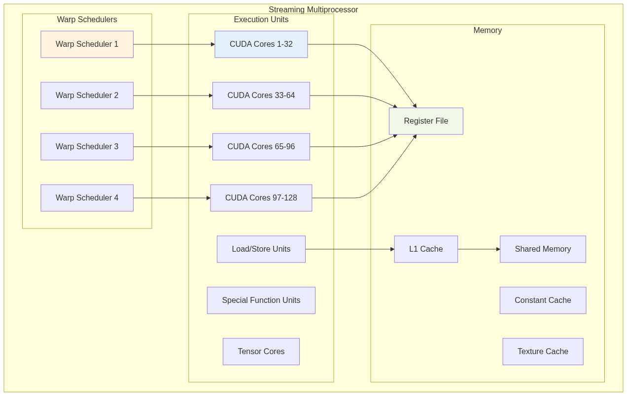
This visualization shows how the hierarchical organization enables massive parallelism while maintaining efficient data flow and resource utilization.

Further Reading

For deeper understanding of GPU architecture and parallel computing:

• NVIDIA CUDA Programming Guide
• “GPU Gems” series by NVIDIA
• “Heterogeneous Computing with OpenCL” by Gaster et al.
• “Programming Massively Parallel Processors” by Kirk and Hwu
• “Real-Time Rendering” by Akenine-Möller et al.

Conclusion

Modern GPU architecture represents a fascinating convergence of parallel processing capabilities, sophisticated memory hierarchies, and specialized computational units. Through our detailed exploration of physical architecture, computational models, and practical implementations, we’ve seen how GPUs achieve their remarkable performance in specific workloads.

Key takeaways:

• GPUs excel at parallel processing through their SIMD/SIMT architecture.
• Memory hierarchy and bandwidth are crucial for GPU performance.
• Specialized cores (Tensor, RT) enable efficient handling of specific computations.
• Modern GPU architecture continues to evolve, particularly in areas like AI and ray tracing.

The future of GPU architecture promises even more exciting developments, particularly in areas like real-time ray tracing, AI acceleration, and general-purpose computing. Understanding these fundamentals provides a solid foundation for leveraging these powerful processors in various applications, from gaming to scientific computing.